Video Lesson

Lesson objective

Dear learners,

At the end of the lesson you will be able to

• Derive and apply the equations of uniformly accelerated motion in 1D.
• Solve various problems of uniformly accelerated motion in 1d.

Brainstorming question

• After revising what you have learnt in grades 9 and 10 about motion in a straight line and uniformly accelerated motion discuss about the following questions in group and present your group’s answers to the class.
• Define the terms position, distance, displacement, speed, and velocity in motion.
• Explain the relationship between position and displacement, distance and displacement, distance and speed, displacement and velocity, average velocity and instantaneous velocity.
• When do we say an object is accelerating?
• How will it be possible for a car to move but not accelerating?

Key Terms and Concepts

Derivation of equations of motion for uniformly accelerated motion in a straight line.

• Equation of motion is a mathematical formula that describes how a physical system behaves over time.
• The equation of MOTION describes objects and systems’ motion in terms of dynamic variables.
• These equations relate various important parameters of motion such as velocity, displacement, speed, time, and acceleration.
• An object is said to be in motion if it changes its position with respect to the same reference point or frame of reference with time.
• Motion can be described in two ways: Dynamics and Kinematics 
• Dynamics deals with the study of the motion of the bodies taking into account the forces which cause the motion in the bodies.
• Kinematics deals with studying the motion of the bodies without taking into account the cause of the motion in the bodies.
• At constant acceleration, the kinematic equations of motion are referred to as the SUVAT equations, arising from the definitions of kinematic quantities: displacement (s), initial velocity (u), final velocity (v), acceleration (a), and time (t).
• The symbols used have the following meanings:
• s = displacement , v_i = initial velocity ,
• V_f = final velocity , t = time for the acceleration , and a = acceleration
• Directly from the definition of acceleration, we get
• $\overrightarrow{a}=\frac{V_{f}-V_{i}}{t}$
• $V_{f}=V_{i}+at $——————–Equation 1
• From the definition of average velocity, we get
• $S=V_{av}t$ ,but for uniformly accelerated motion,
• $V_{av}=\frac{V_{i}+V_{f}}{2}$——–Equation 2
• Remember that average velocity and instantaneous velocities are different. Instantaneous velocity is the velocity at a particular instant of time, but average velocity is the velocity that represents a motion in a certain interval of time.
• Substituting this equation of average velocity into the above equation of displacement
• $S=\left( \frac{V_{i}+V_{f}}{2} \right)t$——Equation 3
• By substituting for final velocity from equation 1 into equation 2 and rearranging gives
• $S=\left( \frac{V_{i}+V_{f}}{2} \right)t$=$\left( \frac{V_{i}+V_{i}+at}{2} \right)t$
• $S=V_{i}t+\frac{1}{2}a^{}t^{2}$————-Equation 4
• Instead of final velocity if we substitute for initial velocity into equation 2 and rearranging gives
• $S=V_{f}t-\frac{1}{2}a^{}t^{2}$———–Equation 5
• Rearranging equation 1 for time (t) and substituting into equation 2 gives
• $S=\left( \frac{V_{i}+V_{f}}{2} \right)t$=$\left( \frac{V_{i}+V_{f}}{2} \right)\left( \frac{V_{f}-V_{i}}{a} \right)$=$\left( \frac{V_{f}^{2}-V_{i}^{2}}{2a} \right)$
• $V_{f}^{2}=V_{i}^{2}+2as$————-Equation 6
• Note that, the above 6 equations all refer to uniformly accelerated motion in a straight line.
• It means that, they do not apply if the acceleration is changing.

Table 3.1: Kinematics equations for uniformly accelerated motion

Equation	Missing quantity
$V_{f}=V_{i}+at $	Displacement (S )
$V_{av}=\frac{V_{i}+V_{f}}{2}$	Displacement (s), acceleration (a), and time (t)
$S=\left( \frac{V_{i}+V_{f}}{2} \right)t$	Acceleration (a)
$S=V_{i}t+\frac{1}{2}a^{}t^{2}$	Final velocity (V f )
$S=V_{f}t-\frac{1}{2}a^{}t^{2}$	Initial velocity ( Vi )
$V_{f}^{2}=V_{i}^{2}+2as$	Time (t )

• Note that the above equations are vector equations,
• it means that we need to take of the direction of the quantities to be added.
• If they are in the same direction we add, but
• if they point in opposite directions we subtract.

Example 2.1

An object dropped from a cliff falls with a constant acceleration of 10 m/s². Find its speed 5 s after it was dropped.

Solution

v=u+at

Here u=0, a=10 m/s², t= 5 s

v=10×5=50m/s

Example 2.2

A bike accelerates uniformly from rest to a speed of 7.10 m/s over a distance of 35.4 m. Determine the acceleration of the bike. 

Given

u = 0 m/s

v = 7.10 m/s

s = 35.4 m

Required

a = ?

Solution

According to the Third Equation of Motion: 

 v² = u² + 2as

(7.10)2 = (0)2 + 2*(a)*(35.4)

50.4 = (70.8)*a

(50.4)/(70.8) = a

a = 0.712 m/s²

Example 2.3

An engineer is designing the runway for an airport. Of the planes that will use the airport, the lowest acceleration rate will likely be 3 m/s². The takeoff speed for this plane will be 65 m/s. Assuming this minimum acceleration, what is the minimum allowed length for the runway?

Given

u = 0 m/s

v = 65 m/s

a = 3 m/s²

Required

s = ?

Solution

As per the Third Equation of Motion

v² =u²+ 2as

(65)² = (0)² + 2*(3)*s

4225 = (6)*s

(4225)/(6) = s

d = 704 m

• Note that all negative accelerations are not always decelerations.
• Negative acceleration can also occur due to the change in direction with respect to a certain fixed reference point.

Determining the stopping distance of a vehicle

• When brakes are applied to a moving vehicle, the distance it travels before stopping is called stopping distance.
• Calculating stopping distance is important for avoiding potential hazardous situations.
• There are many factors that can affect the stopping distance of a moving vehicle. Here are some;

1. Speed of the vehicle
2. Weight of the vehicle
3. Road conditions (slick, icy, snow, dry, wet)
4. Vehicle brake conditions (old or worn pads and rotors)
5. Braking technology in the vehicle
6. Tire conditions

• This leads us to the actual formula for working out braking distances. The formula is based on the velocity (speed) of the vehicle and the coefficient of friction between the wheels and the road ($\mu$ ).
• $\left( S_{break} \right)=\frac{V^{2}}{2a}=\frac{V^{2}}{2g\mu}$
• This is because, for a car coming to a stop due to friction:
• Experiments have a= µ g. shown that for dry roads, the coefficient of friction is about 0.7, and for wet roads it is about 0.4.
• The stopping distance is then the sum of reaction distance and braking distance.

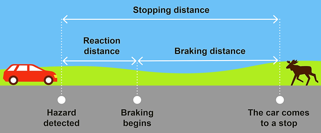
Figure 2.2 stopping distance of a vehicle

• The reaction distance is the distance you travel from the point of detecting a hazard until you begin braking or swerving.
• The time between being where we first start measuring, and where the car begins braking, is called the reaction time.
• As an equation, looking at the car’s speed, 𝑣, the distance 𝑣 it travels over a period of time 𝑣 is:
• The reaction distance = The car’s speed$\ast$ reaction time.
• Reaction distance s_r= vt
• Stopping distance = reaction distance + braking distance
• Stoppind distance = vt+$\frac{V^{2}}{2g\mu}$